Surface processes model¶

The whole landscape evolution can basically be represented in a single equation:

\[\frac{\partial z}{\partial t} = U - E - \nabla \cdot q_s\]

All landscape must obey this fundamental statement about sediment transport. In this equation \(\frac{\partial z}{\partial t}\) is the change in surface elevation, \(U\) is the uplift rate, \(E\) is the erosion rate and \(\nabla \cdot q_s\) is the sediment flux divergence.

The erosion rate \(E\) corresponds to sediment production from weathering and bedrock erosion by glacier, wind, water. The sediment fluxes is transported by hillslope and fluvial transport processes.

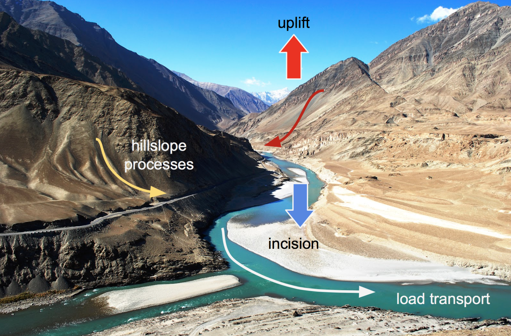
Fig. 60 Surface processes are acting everywhere we have relief, but more obviously in mountain regions. In response to tectonic uplift, rivers incise into bedrock and insure the progressive lowering of the base level for hillslope processes to take place. Rivers also transport the eroded materials to the sedimentary basin.

Note

Many geomorphological applications have demonstrated the usefulness of these models, whose predictions help researchers test simple to complex hypotheses on the nature of landscape evolution. Surface processes models (SPMs) also provide connection between small scale, measurable processes and their long-term geomorphic implications.

Preamble¶

The roots of landscape evolution theory can be found in the pioneering work of Gilbert (1877), who proposed a set of hypotheses to relate various landforms to the mechanisms of weathering, erosion and sediment transport. The first quantitative models appeared later in the 1960s (e.g., Culling, 1960; Scheidegger, 1961; Ahnert, 1970; Kirkby, 1971). These models formalise the concepts of Gilbert (1877) to the development of hillslope profiles. A few years later, these models were extended to two dimensions, although still focused on hillslope morphology.

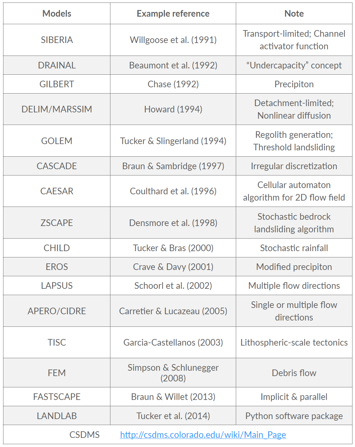
Fig. 61 Partial list of existing landscape evolution models.

During the last two decades, as computers continued to get faster, a number of sophisticated numerical SPMs have been developed, mainly focusing on watershed and mountain belt evolution. Both hillslope and fluvial processes are involved in these models, which differ from each other by the parameterisation of these processes and their numerical resolution.

Continuity of mass¶

In the case where there is no distinction between a regolith layer and the bedrock underneath, the mass continuity equations for a column of soil or rock is expressed as:

\[\frac{\partial z}{\partial t} = U - \nabla \cdot q_s\]

where the elevation \(z\) (m) is measured vertically, \(q_s\) is the total downhill soil flux, \(\nabla \cdot\) is the spatial divergence operator and \(U\) (m/yr) is a source term that can either represent the rate of incision of channel streams at the hillslope boundaries or uniform uplift.

Sediment transport¶

To describe the rates of sediment erosion/transport/deposition, several approaches have been proposed. In its simplest formalism a detachment-limited equation is often used.

Detachment-limited model¶

The soil transport rate per unit width by flowing water, \(q_r\), is modelled as a power function of topographic gradient \(\nabla z\) and surface water discharge per unit width \(q_w\) (m2/yr):

\[q_r = − \kappa_r q_w^m \nabla z^n\]

This detachment-limited incision rate, which is calculated as a power law function of fluvial discharge only applies where channel slope is positive. This brings the following relatioship:

\[\frac{\partial z}{\partial t} = − \kappa_r q_w^m \nabla z^n\]

This expression corresponds to a simplified form of the usual expression of sediment transport by water flow, in which the transport rate is assumed to be equal to the local carrying capacity, which is itself a function of boundary shear stress or stream power per unit width. We consider additionally no threshold for particle entrainment. Generally, the exponents m and n have values between 1 and 2.

Hillslope processes¶

In its most simple form, the parameterisation of hillslope transport is based on a linear dependence to the topographic gradient. This linear law has in fact been used to represent a variety of transport processes such as creep, biogenic activity or rain splash.

Downslope simple creep is commonly regarded as operating in a shallow superficial layer and is defined as:

\[q_d = − \kappa_d \nabla z\]

Note that because of the multi-process parameterisation of soil transport, the coefficient \(\kappa_d\) is also scale-dependent, like the \(\kappa\)-scale parameters of the other stream power law defined above.

Incision laws overview¶

Important

Several formulations of river incision have been proposed to account for long term evolution of fluvial system. These formulations describe different erosional behaviours ranging from detachment-limited incision, governed by bed resistance to erosion, to transport-limited incision, governed by flow capacity to transport sediment available on the bed.

As we already discussed, mathematical representation of erosion processes in these formulations is often assumed to follow a stream power law. These relatively simple approaches have two main advantages. First, they have been shown to approximate the first order kinematics of landscape evolution across geologically relevant timescales (> \(10^4\) years). Second, neither the details of long term catchment hydrology nor the complexity of sediment mobilisation dynamics are required. However, other formulations are sometimes necessary when addressing specific aspects of landscape evolution.

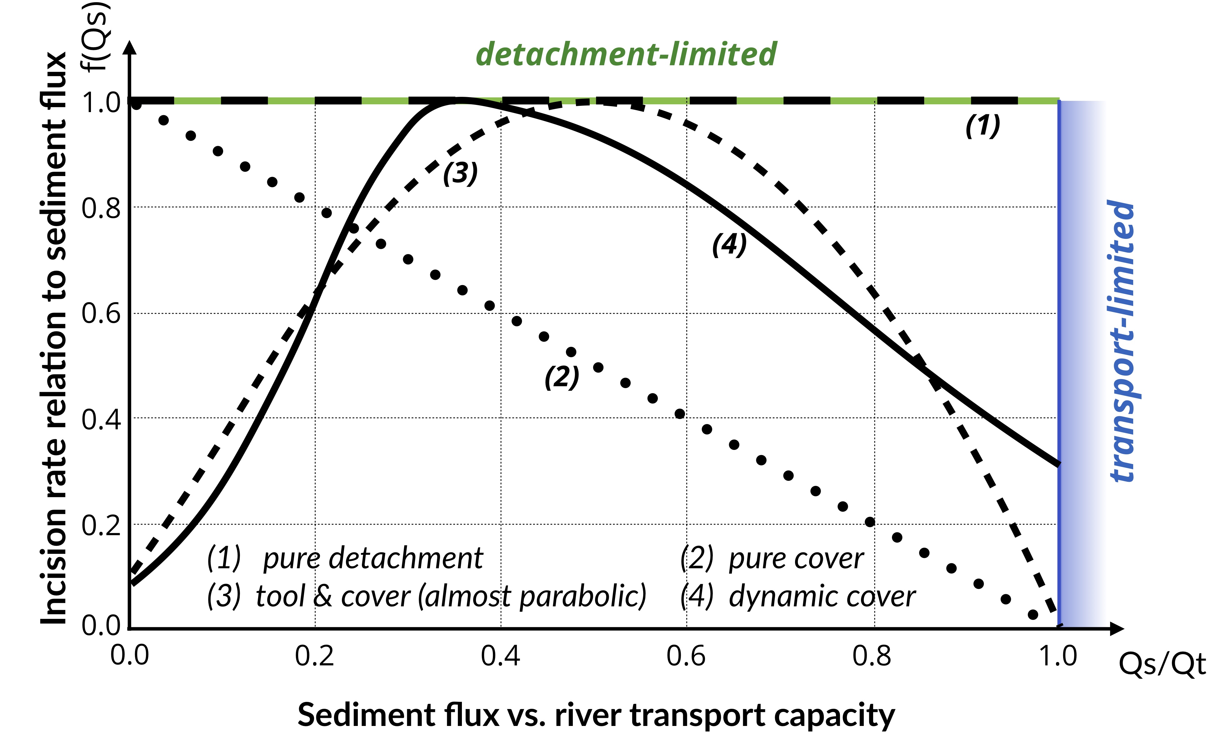
Fig. 62 Model space for stream power-based incision laws. It shows the dependence of river incision rate on sediment flux (adapted from Hobley et al., 2011).

Detachment-limited¶

The simplest law to simulate fluvial incision is based on the detachment-limited stream power law (option 1, in the above figure), in which erosion rate depends on drainage area \(A\), net precipitation \(P\) and local slope \(S\) and takes the form:

\[I = − \kappa_d P^l (PA)^m S^n\]

\(\kappa_d\) is a dimensional coefficient describing the erodibility of the channel bed as a function of rock strength, bed roughness and climate, \(l\), \(m\) and \(n\) are dimensionless positive constants.

Default formulation assumes \(l = 0\), \(m = 0.5\) and \(n = 1\). The precipitation exponent \(l\) allows for representation of climate-dependent chemical weathering of river bed across non-uniform rainfall. In this model sediment deposition occurs solely in topographically closed depression and offshore.

Transport-limited¶

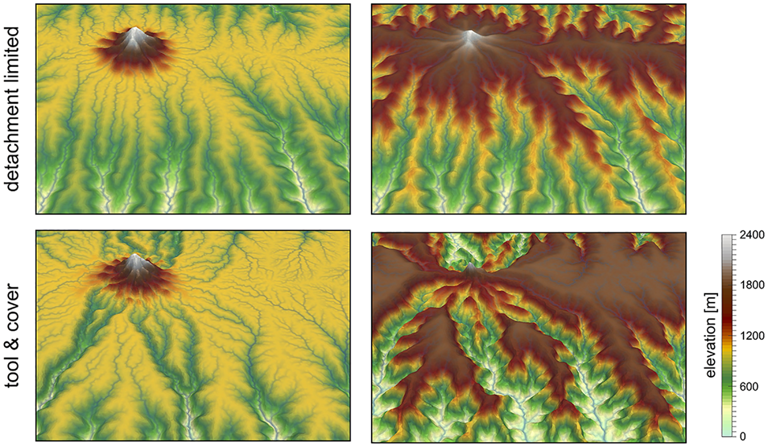
Fig. 63 Illustration of the impact of detachment versus transport limited (tool & cover option 3) formulations on landscape dynamics. Evolution of dissection of an uplifting landscape composed of a flat surfaces dotted with an isolated peak, after 5 and 9 Ma of dissection. The modeling shows how the abundant bedload shed by the isolated peak boosts incision along the receiving streams (tool effect).

Here, volumetric sediment transport capacity (\(Q_t\)) is defined using a power law function of unit stream power:

\[Q_t = − \kappa_t (PA)^m_t S^n_t\]

where \(\kappa_t\) is a dimensional coefficient describing the transportability of channel sediment and \(m_t\) and \(n_t\) are dimensionless positive constants. In this equation, the threshold of motion (the critical shear stress) is assumed to be negligible.

An additional term is now introduced in the stream power model:

\[I = − \kappa f(Q_s) (PA)^m S^n\]

with \(f(Q_s)\) representing a variety of plausible models for the dependence of river incision rate on sediment flux \(Q_s\). In the standard detachment-limited, \(f(Q_s)\) is equal to unity, which corresponds to cases where \(Qs << Qt\). All sediment is dispersed downstream and the incision limiting factor is bedrock erodibility.

Addition of the transport-limited function results in the fact that, where sediment flux equals or exceeds transport capacity (\(Q_s/Q_t \ge 1\)) the system becomes transport-limited and depositional if \(Qs/Qt > 1\). In this model the time-evolving distribution of erosion and sedimentation, is affected by the distribution of detachment-limited and transport-limited reaches, which is controlled by the respective values of \(\kappa_d\) and \(\kappa_t\).

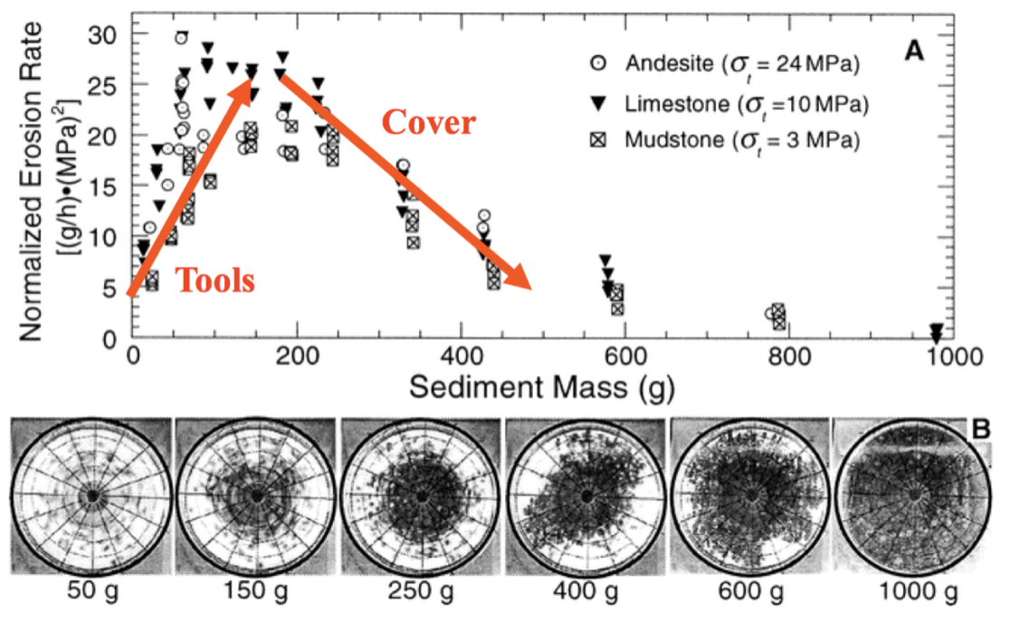
Fig. 64 Experimental study of bedrock abrasion by saltating particles (Sklar & Dietrich, 2001). The tool effect corresponds to impacting particles that remove rock, the more particles in the flow the higher the erosion rate. The cover effect corresponds to the effect of bed protection related to the amount of particles within the flow. The more particles the smaller the erosion rates.

The transition from one behaviour to the other can be treated either abruptly, progressively, through the use of one of the following formulations:

Linear decline: This model belongs to the undercapacity family of models: it assumes that stream incision represents the expenditure of the energy in excess of that needed to transport the bypassing sediment load. Stream incision potential decreases linearly from a maximum where sediment flux is negligible, to zero where sediment flux equals transport capacity (option 2).
Almost parabolic: Both qualitative and experimental observations have shown that sediment flux has a dual role in the river bed incision. First, when sediment flux is low relative to carrying capacity, erosion potential increases with sediment flux (tool effect: bedrock abrasion and plucking). Then, with increased sediment flux, erosion is inhibited (cover effect: sediments protect the bed from impacts by saltating particles) (option 3).
Dynamic cover: Typically gravel-river beds have an armoured layer of coarse grains on the surface, which acts to protect finer particles underneath from erosion. To account for sediment and spatial heterogeneity in the armouring of the river bed, Turowski et al. proposed a modified form of the ‘almost parabolic’ model that better estimates the original Sklar and Dietrich experiments (option 4).

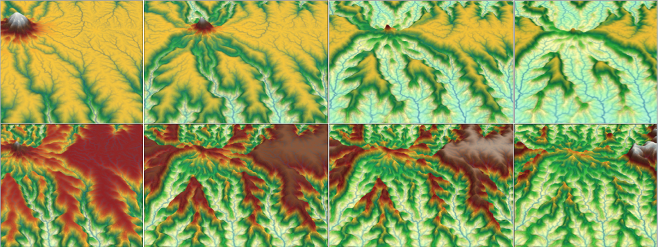
Fig. 65 Preferential erosion and low relief preservation.

Step-by-step approach to landscape evolution model¶

Step 1: Flow directions¶

Important

Landscape evolution applications generally require computing the drainage network of a terrain, consisting of the flow direction and flow accumulation. Intuitively, they are the path that water flows through the terrain and the amount of water that flows into each terrain cell supposing that each cell receives a rain drop

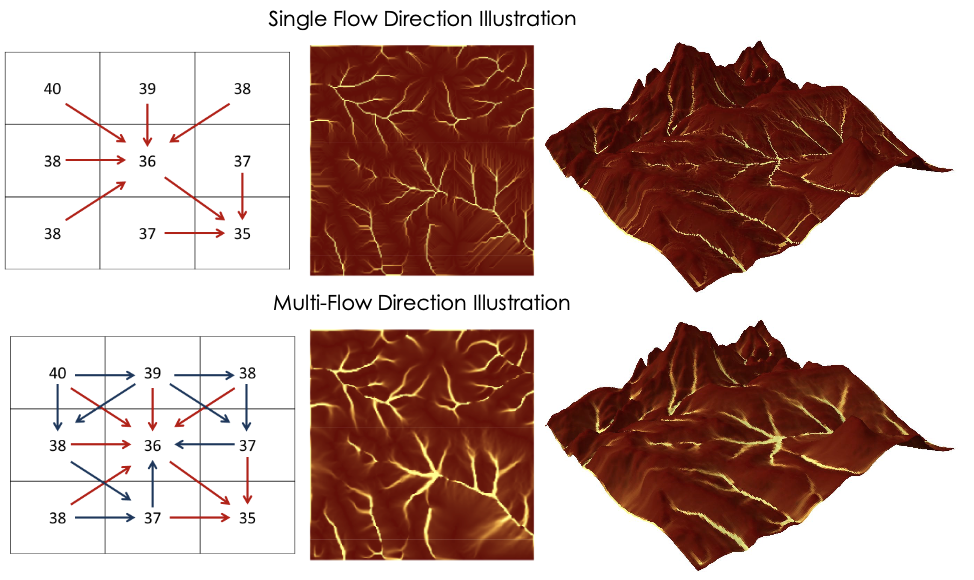
Fig. 66 Different approaches (SFD & MFD) to estimate flow directions.

The drainage network of a terrain delineates the path that water flows through the terrain (the flow direction) and the amount of water that flows into each terrain cell (the flow accumulation). The flow direction problem is to assign flow directions to all cells in the terrain such that the following three conditions are fulfilled:

Every cell has at least one flow direction;
No cyclic flow paths exist; and
Every cell in the terrain has a flow path to the edge of the terrain.

The flow direction can be modelled considering single flow direction (SFD) or multiple flow directions (MFD). In SFD, each terrain cell is assigned a direction towards the steepest downslope neighbour, while in MFD, each cell has directions to all downslope neighbours. The use of SFD or MFD is essentially a modeling choice since the computational complexity of the flow routing problem is the same in both models.

Step 2: Pit filling¶

Important

The major challenge in the process is the flow routing in local minimum and flat areas. A local minimum is a cell with no downslope neighbour and a flat area is a set of adjacent cells with a same elevation.

A neighbour cell of c is called a downslope neighbour if it has a strictly lower elevation than c. A cell in a flat area that has a downslope neighbour is called a spill-point. Also, a flat area can be classified as a plateau or a sink where the plateau has a spill point and a sink doesn’t. Intuitively, water will accumulate in a sink until it fills up and water flows out of it, while in the plateau the water should flow towards spill points.

Usually, most drainage network computation methods use a preprocessing step to remove the sinks and the flat areas. Initially, the elevation of the cells belonging to a sink are increased to transform it into a plateau. Next, the flow directions on the plateau are assigned to ensure that there is a path from each cell to the nearest spill point.

Pit-filling exercise

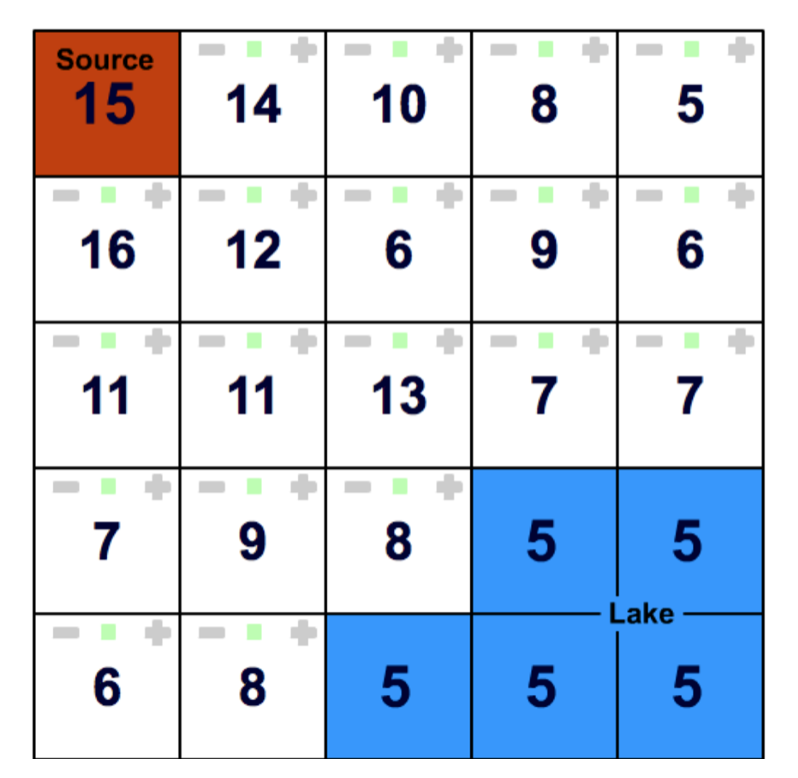
Fig. 67 Digital elevation grid showing each cell elevation.

Starting from the source cell and considering a single flow direction (SFD) approach answer these questions:

There is a pit in this DEM, identify it, which value is required to fill it and allow the flow to keep moving downslope?
Where is the water from the source entering the lake?

Step 3: Flow accumulation and erosion¶

After obtaining the flow direction, the next step consists in computing the flow accumulation in each terrain cell, that is, the amount of water flowing to each cell supposing that all cells receive a drop of water and this water follows the direction obtained in the previous step.

Once the flow accumulation has been computed for a particular topography, the erosion is then estimated using one of the incision laws defined in the previous section and requires at least the estimation of the slope based on the flow direction. The erosion values are finally used to change the topography elevations and the model moves forward in time.

At the next iteration, steps 1 to 3 are applied on the new elevation grid allowing to simulate landscape evolution over time.